Hi everyone. In my previous post, I started by apologizing for the delay in posting; I will begin today with both a similar apology and also a similar excuse. I’ve been CONTINUING to work on online classwork, completing the 3rd and 4th (final two) courses in the MITx PRO Quantum Computing Fundamentals curriculum. Interestingly, since I last posted the 3rd and 4th courses don’t seem to be part of the training any more. I’m not sure why that is, but I can say these courses on “Quantum Computing Realities” are a step more detailed, focusing on the physical limitations of current quantum technology, namely noise, and the workarounds. Both the math and use cases examples are less about practical application and more for those interested in understanding the second order physics. On to the update…
In my previous post, I revisited the concept of superposition, in which quantum bits (qubits) can supposedly be both 0 and 1 at the same time. I will argue this is a bit theatrical. In reality, they can be “between” 0 and 1 states, bring forth the concept of “maybe” or partiality to quantum computing that does not exist with binary logic.
We reintroduced the Block Sphere, where the state of a given qubit is logically expressed as it’s position on the sphere and better conceptualized as a vector than a simple 0 or 1 state.
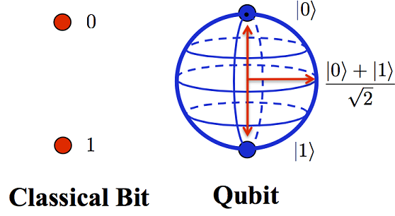
The state at the top pole of the Block sphere is referred to as |0>, the state at the bottom pole as |1>, the state at the middle (not going into the math here) as (|0> + |1>) / √2. Voila!… 0 and 1 at the same time. Again, it’s not so much that the qubit is in both states at the same time, it’s that it’s somewhere in between, or indeterminate. NOTE: After thinking about the last I want to emphasize that the Bloch Sphere representation is a logical representation. They are many physical ways to represent this behavior, which would make a good future post.
The power of a quantum computer comes from the ability to perform tasks on this “in-between” state, achieving a degree of parallelism that does not exist with classical computers. One place where quantum computing becomes interesting is, should we measure the state of the qubit, we will measure a 0 or 1, but we can’t predict which get with the exception we tend to get either state with equal probability.
I offered to demonstrate superposition, here goes. I will be using the IBM Q Experience online simulation tools.
Without going too far into the details, a basic first-step to modeling a quantum circuit is to initialize the bits to a superposition. This is done, typically, but setting all the bits to a known |0> state, then applying what’s called a Hadamard gate, represented by the letter H, which sets the qubit midway between |0> and |1> (drastically oversimplified). To further illustrate, I will introduce what’s called a C-NOT gate which logically behaves like a classic XOR gate. Here’s the truth table for a reminder:
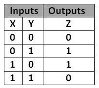
In a C-NOT gate, the first bit (X) “controls” the second bit (Y), inverting the second bit (Y) when the first bit is set to 1.
Here’s what that circuit look like in the simulator.
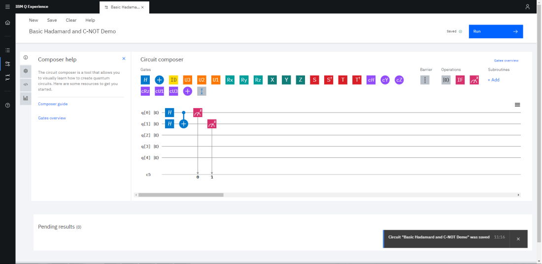
Again, the Hadamard gate sets the [0] and [1] bits to the “in-between” state. When we measure a bit after a Hadamard gate, we’ll get a 0 or a 1, but we won’t known which. This applies directly to the [0] bit as we are measuring the output of the H gate directly. The [1] bit is the controlled bit and we would expect a truth table like the one show previously – i.e. when bit [0] is 1, we will expect the [1] bit to become inverted.
Here are the simulated results:
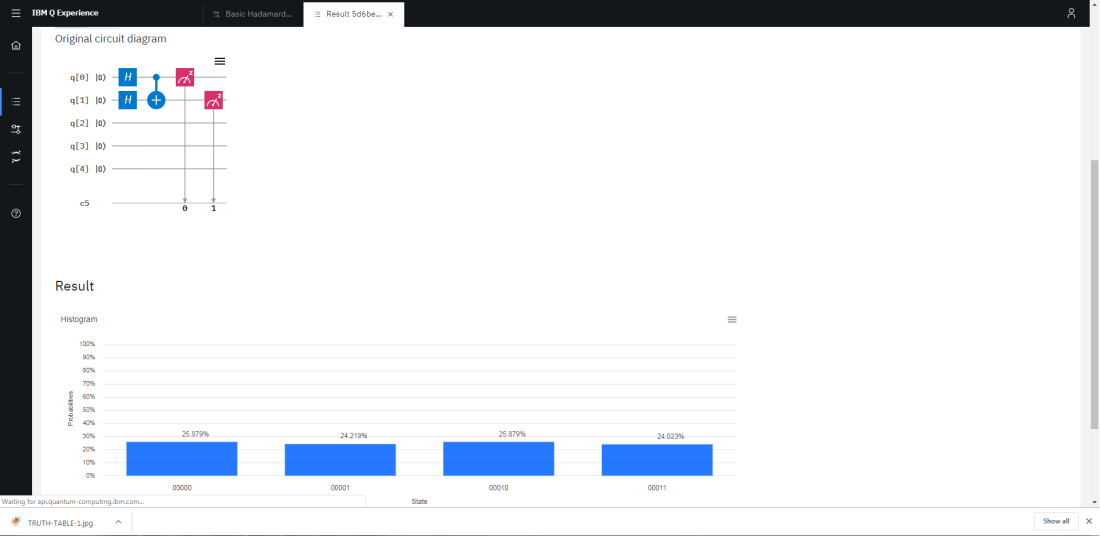
As you can see, we get the expected results where bit [0] is 0 half of the time and 1 the other half. And within each of those, the [1] is appropriately inverted (or not) depending on the value of [0]. Each row in the truth table accordingly is shown at about 25% probability of occurring.
More sophisticated quantum algorithms leverage this behavior with more meaningful circuits. Finding a simple enough example algorithm to show here remains part of the journey.
